REINFORCEjs

Setup

This demo is a modification of PuckWorld:

• The state space is now large and continuous: The agent observes its own location (x,y), velocity (vx,vy), the locations of the green target, and the red target (total of 8 numbers).
• There are 4 actions available to the agent: To apply thrusters to the left, right, up and down. This gives the agent control over its velocity.
• The PuckWorld dynamics integrate the velocity of the agent to change its position. The green target moves once in a while to a random location. The red target always slowly follows the agent.
• The reward awarded to the agent is based on its distance to the green target (low is good). However, if the agent is in the vicinity of the red target (inside the disk), the agent gets a negative reward proportional to its distance to the red target.

The optimal strategy for the agent is to always go towards the green target (this is the regular PuckWorld), but to also avoid the red target's area of effect. This makes things more interesting because the agent has to learn to avoid it. Also, sometimes it's fun to watch the red target corner the agent. In this case, the optimal thing to do is to temporarily pay the price to zoom by quickly and away, rather than getting cornered and paying much more reward price when that happens.

Interface: The current reward experienced by the agent is shown as its color (green = high, red = low). The action taken by the agent (the medium-sized circle moving around) is shown by the arrow.

Deep Q Learning

We're going to extend the Temporal Difference Learning (Q-Learning) to continuous state spaces. In the previos demo we've estimated the Q learning function \(Q(s,a)\) as a lookup table. Now, we are going to use a function approximator to model \(Q(s,a) = f_{\theta}(s,a)\), where \(\theta\) are some parameters (e.g. weights and biases of a neurons in a network). However, as we will see everything else remains exactly the same. The first paper that showed impressive results with this approach was Playing Atari with Deep Reinforcement Learning at NIPS workshop in 2013, and more recently the Nature paper Human-level control through deep reinforcement learning, both by Mnih et al. However, more impressive than what we'll develop here, their function \(f_{\theta,a}\) was an entire Convolutional Neural Network that looked at the raw pixels of Atari game console. It's hard to get all that to work in JS :(

Recall that in Q-Learning we had training data that is a single chain of \(s_t, a_t, r_t, s_{t+1}, a_{t+1}, r_{t+1}, s_{t+2}, \ldots \) where the states \(s\) and the rewards \(r\) are samples from the environment dynamics, and the actions \(a\) are sampled from the agent's policy \(a_t \sim \pi(a \mid s_t)\). The agent's policy in Q-learning is to execute the action that is currently estimated to have the highest value (\( \pi(a \mid s) = \arg\max_a Q(s,a) \)), or with a probability \(\epsilon\) to take a random action to ensure some exploration. The Q-Learning update at each time step then had the following form:

$$ Q(s_t, a_t) \leftarrow Q(s_t, a_t) + \alpha \left[ r_t + \gamma \max_a Q(s_{t+1}, a) - Q(s_t, a_t) \right] $$

As mentioned, this equation is describing a regular Stochastic Gradient Descent update with learning rate \(\alpha\) and the loss function at time \(t\):

$$ L_t = (r_t + \gamma \max_a Q(s_{t+1}, a) - Q(s_t, a_t))^2 $$

Here \(y = r_t + \gamma \max_a Q(s_{t+1}, a)\) is thought of as a scalar-valued fixed target, while we backpropagate through the neural network that produced the prediction \(f_{\theta} = Q(s_t,a_t)\). Note that the loss has a standard L2 norm regression form, and that we nudge the parameter vector \(\theta\) in a way that makes the computed \(Q(s,a)\) slightly closer to what it should be (i.e. to satisfy the Bellman equation). This softly encourages the constraint that the reward should be properly diffused, in expectation, backwards through the environment dynamics and the agent's policy.

In other words, Deep Q Learning is a 1-dimensional regression problem with a vanilla neural network, solved with vanilla stochastic gradient descent, except our training data is not fixed but generated by interacting with the environment.

Bells and Whistles

There are several bells and whistles that make Q Learning with function approximation tracktable in practical problems:

Modeling Q(s,a). First, as mentioned we are using a function approximator to model the Q function: \(Q(s,a) = f_{\theta}(s,a)\). The natural approach to take is to perhaps have a neural network that takes as inputs the state vector \(s\) and an action vector \(a\) (e.g. encoded with a 1-of-k indicator vector), and output a single number that gives \(Q(s,a)\). However, this approach leads to a practical problem because the policy of the agent is to take an action that maximizes Q, that is: \( \pi(a \mid s) = \arg\max_a Q(s,a) \). Therefore, with this naive approach, when the agent wants to produce an action we'd have to iterate over all actions, evaluate Q for each one and take the action that gave the highest Q.

A better idea is to instead predict the value \(Q(s,a)\) as a neural network that only takes the state \(s\), and produces multiple output, each interpreted as the Q value of taking that action in the given state. This way, deciding what action to take reduces to performing a single forward pass of the network and finding the argmax action. A diagram may help get the idea across:

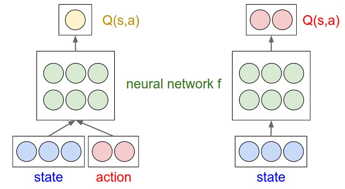
Simple example with 3-dimensional state space (blue) and 2 possible actions (red). Green nodes are neurons of a neural network f. Left: A naive approach in which it takes multiple forward passes to find the argmax action. Right: A more efficient approach where the Q(s,a) computation is effectively shared among the neurons in the network. Only a single forward pass is required to find the best action to take in any given state.

Formulated in this way, the update algorithm becomes:

1. Experience a \(s_t, a_t, r_t, s_{t+1}\) transition in the environment.
2. Forward \(s_{t+1}\) to evaluate the (fixed) target \(y = r_t + \gamma \max_a f_{\theta}(s_{t+1})\).
3. Forward \(f_{\theta}(s_t)\) and apply L2 regression loss on the dimension \(a_t\) of the output which we want to equal to \(y\). Due to the L2 loss, the gradient has a simple form where the predicted value is simply subtracted from \(y\). The output dimensions corresponding to the other actions have zero gradient.
4. Backpropagate the gradient and perform a parameter update.

Experience Replay Memory. An important contribution of the Mnih et al. papers was to suggest an experience replay memory. This is loosely inspired by the brain, and in particular the way it syncs memory traces in the hippocampus with the cortex. What this amounts to is that instead of performing an update and then throwing away the experience tuple \(s_t, a_t, r_t, s_{t+1}\), we keep it around and effectively build up a training set of experiences. Then, we don't learn based on the new experience that comes in at time \(t\), but instead sample random expriences from the replay memory and perform an update on each sample. Again, this is exactly as if we were training a Neural Net with SGD on a dataset in a regular Machine Learning setup, except here the dataset is a result of agent interaction. This feature has the effect of removing correlations in the observed state,action,reward sequence and reduces gradual drift and forgetting. The algorihm hence becomes:

1. Experience \(s_t, a_t, r_t, s_{t+1}\) in the environment and add it to the training dataset \(\mathcal{D}\). If the size of \(\mathcal{D}\) is greater than some threshold, start replacing old experiences.
2. Sample N experiences from \(\mathcal{D}\) at random and update the Q function.

Clamping TD Error. Another interesting feature is to clamp the TD Error gradient at some fixed maximum value. That is, if the TD Error \(r_t + \gamma \max_a Q(s_{t+1}, a) - Q(s_t, a_t)\) is greater in magnitude then some threshold spec.tderror_clamp, then we cap it at that value. This makes the learning more robust to outliers and has the interpretation of using Huber loss, which is an L2 penalty in a small region around the target value and an L1 penalty further away.

Periodic Target Q Value Updates. The last modification suggested in Mnih et al. also aims to reduce correlations between updates and the immediately undertaken behavior. The idea is to freeze the Q network once in a while into a frozen, copied network \(\hat{Q}\) which is used to only compute the targets. This target network is once in a while updated to the actual current \(Q\) network. That is, we use the target network \(r_t + \gamma \max_a \hat{Q}(s_{t+1},a)\) to compute the target, and \(Q\) to evaluate the \(Q(s_t, a_t)\) part. In terms of the implementation, this requires one additional line of code where we every now and then we sync \(\hat{Q} \leftarrow Q\). I played around with this idea but at least on my simple toy examples I did not find it to give a substantial benefit, so I took it out of REINFORCEjs in the current implementation for sake of brevity.

REINFORCEjs API use of DQN

If you'd like to use REINFORCEjs DQN in your application, define an env object that has the following methods:

• env.getNumStates() returns an integer for the dimensionality of the state feature space
• env.getMaxNumActions() returns an integer with the number of actions the agent can use

This seems kind of silly and the name getNumStates is a bit of a misnomer because it refers to the size of the state feature vector, not the raw number of unique states, but I chose this interface so that it is consistent with the tabular TD code and DP method. Similar to the tabular TD agent, the IO with the agent has an extremely simple interface:

// create environment
var env = {};
env.getNumStates = function() { return 8; }
env.getMaxNumActions = function() { return 4; }

// create the agent, yay!
var spec = { alpha: 0.01 } // see full options on top of this page
agent = new RL.DQNAgent(env, spec); 

setInterval(function(){ // start the learning loop
  var action = agent.act(s); // s is an array of length 8
  // execute action in environment and get the reward
  agent.learn(reward); // the agent improves its Q,policy,model, etc. reward is a float
}, 0);

As for the available parameters in the DQN agent spec:

• spec.gamma is the discount rate. When it is zero, the agent will be maximally greedy and won't plan ahead at all. It will grab all the reward it can get right away. For example, children that fail the marshmallow experiment have a very low gamma. This parameter goes up to 1, but cannot be greater than or equal to 1 (this would make the discounted reward infinite).
• spec.epsilon controls the epsilon-greedy policy. High epsilon (up to 1) will cause the agent to take more random actions. It is a good idea to start with a high epsilon (e.g. 0.2 or even a bit higher) and decay it over time to be lower (e.g. 0.05).
• spec.num_hidden_units: currently the DQN agent is hardcoded to use a neural net with one hidden layer, the size of which is controlled with this parameter. For each problems you may get away with smaller networks.
• spec.alpha controls the learning rate. Everyone sets this by trial and error and that's pretty much the best thing we have.
• spec.experience_add_every: REINFORCEjs won't add a new experience to replay every single frame to try to conserve resources and get more variaty. You can turn this off by setting this parameter to 1. Default = 5
• spec.experience_size: size of memory. More difficult problems may need bigger memory
• spec.learning_steps_per_iteration: the more the better, but slower. Default = 20
• spec.tderror_clamp: for robustness, clamp the TD Errror gradient at this value.

Pros and Cons

The very nice property of DQN agents is that the I/O interface is quite generic and very simple: The agent accepts state vectors, produces discrete actions, and learns from relatively arbitrary agents. However, there are several things to keep in mind when applying this agent in practice:

• If the rewards are very sparse in the environment the agent will have trouble learning. Right now there is no priority sweeping support, but one might imagine oversampling experience that have high TD errors. It's not clear how this can be done in most principled way. Similarly, there are no eligibility traces right now though this could be added with a few modifications in future versions.
• The exploration is rather naive, since a random action is taken once in a while. If the environment requires longer sequences of precise actions to get a reward, the agent might have a lot of difficulty finding these by chance, and then also learning from them sufficiently.
• DQN only supports a set number of discrete actions and it is not obvious how one can incorporate (high-dimensional) continuous action spaces.

Speaking of high-dimensional continuous action spaces, this is what Policy Gradient Actor Critic methods are quite good at! Head over to the Policy Gradient (PG) demo. (Oops, coming soon...)