If the configuration space is D dimensional, then there are 2D
dimensions in the phase space. It can be shown that in a Hamiltonian
system, the number B of stable and unstable directions is equal, although
B < D is possible.![]() At time
At time ![]() , let
, let ![]() represent D unstable unit vectors,
and let
represent D unstable unit vectors,
and let ![]() represent D stable unit vectors.
For any particular timestep,
it will be convenient if the unstable vectors are orthonormal to each other,
and the stable vectors are orthonormal to each other. However, the stable
and unstable vectors together will not in general form an orthogonal system.
represent D stable unit vectors.
For any particular timestep,
it will be convenient if the unstable vectors are orthonormal to each other,
and the stable vectors are orthonormal to each other. However, the stable
and unstable vectors together will not in general form an orthogonal system.
The vectors are evolved as in the two dimensional case,
except using Gram-Schmidt
orthonormalization to produce two sets of D-orthonormal vectors at each
timestep.
Arbitrary orthonormal bases are chosen, ![]() at time
at time ![]() ,
and
,
and ![]() at time
at time ![]() , and then evolved according to
, and then evolved according to
![]()
At each step i, two Gram-Schmidt
orthonormalizations are done:
one on ![]() to produce
to produce ![]() ,
and another on
,
and another on ![]() to produce
to produce ![]() . After a few e-folding times,
. After a few e-folding times,
![]() points in the most unstable direction at step i,
points in the most unstable direction at step i,
![]() points in the second most unstable direction, etc.
Likewise,
points in the second most unstable direction, etc.
Likewise, ![]() points in the most stable direction at time i,
points in the most stable direction at time i,
![]() points in the second most stable direction, etc.
points in the second most stable direction, etc.
The multidimensional generalization of (10) is the obvious
To convert the 1-step error at step i from phase-space co-ordinates
![]() to the stable and unstable basis
to the stable and unstable basis
![]() ,
one constructs the matrix
,
one constructs the matrix ![]() whose columns are the unstable and stable
unit vectors,
whose columns are the unstable and stable
unit vectors, ![]() ,
and solves the system
,
and solves the system ![]() .
.
From (8) and (16) the equation for the correction co-efficients in the unstable subspace at step i+1 is
![]()
which are projected out along ![]() producing
producing
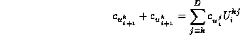
where the scalar ![]() , and the Gram-Schmidt process
ensures
, and the Gram-Schmidt process
ensures ![]() if j < k.
As stated previously, the boundary condition requires the unstable
component of the corrections to be small at timestep S, and their
stable components to be small at timestep 0. For simplicity
we take
if j < k.
As stated previously, the boundary condition requires the unstable
component of the corrections to be small at timestep S, and their
stable components to be small at timestep 0. For simplicity
we take ![]() , as did QT,
and the co-efficients are computed backward using
, as did QT,
and the co-efficients are computed backward using
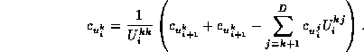
We first solve for ![]() , which does not require knowledge
of the other
, which does not require knowledge
of the other ![]() co-efficients, then solve for
co-efficients, then solve for ![]() ,
etc.
,
etc.
Again from (8) and (16), the equation for the correction co-efficients in the stable subspace at timestep i is
![]()
which are projected out along ![]() producing
producing
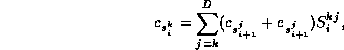
where ![]() , and the Gram-Schmidt process ensures
, and the Gram-Schmidt process ensures ![]() if j < k.
The boundary condition at step 0 is
if j < k.
The boundary condition at step 0 is ![]() ,
and the co-efficients are computed forward using
,
and the co-efficients are computed forward using
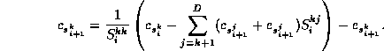
As with the unstable corrections, we first compute ![]() which does not require knowledge of the other
which does not require knowledge of the other ![]() co-efficients, then
we compute
co-efficients, then
we compute ![]() , etc.
, etc.
