

Next: Further work
Up: Some preliminary results of
Previous: One QT-like experiment with
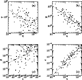
Figure 3.1 is a copy of QT's Figure 6 (copied with permission).

Figure 3.1: Data from QT's Figure 6, used with permission.
Their caption was: ``Results from attempts to shadow noisy orbits in the
unsoftened Plummer model of Fig. 1 [their Figure 1, not included in this
thesis] (each point represents a different orbit): (a) maximum time T
for which the orbit could be shadowed versus the accuracy parameter
 used to generate the orbit; (b) maximum number of time-steps N
for which orbit could be shadowed; (c) shadow distance
  versus
the maximum one-step phase-space error
  in the noisy orbit; (d)
 versus
  . The dashed lines are least-squares fits to the
data.''
See text for a possible explanation of why (b) has less scatter than (a).
In their
text, they mention that part (b) of their figure was included simply
because the scatter was less when they plotted shadow length in
timesteps rather than absolute time. (Recall that they used every
internal timestep of their integrator as a shadow step; thus the shadow steps
would be shorter near close encounters.) They could not provide an adequate
explanation of why the scatter was less in such a graph. What follows
is a tentative explanation.
First, I assume that there are two distinct error magnification
processes effective in N-body systems: one is magnification due
to the global potential, and the other, a much higher magnification
that acts much less frequently, is due to collisional encounters. Thus, if we were to plot successive times at which a doubling (or
e-folding) occurs, the inter-doubling times would be shorter near
close encounters than far from them. Second, different solutions obviously
have their close encounters at different times in their evolutions.
Third, define pseudo-time to progress in units such that the
changing doubling times occur at constant intervals in pseudo-time.
The result is that pseudo-time speeds up near close encounters, in
comparison to real time. Since glitches occur more frequently near
close encounters in real time, glitches will occur at a more uniform
rate in pseudo-time. Finally, the dynamic timesteps used by QT's
integrator will more uniformly follow pseudo-time than does real time,
since it uses small timesteps near close encounters. In other
words, the scatter of glitch occurrence (i.e., end of a shadow that
follows the noisy orbit) is less in pseudo-time (and therefore in
integration timesteps) than in real time. This may explain why
QT's graph 6(b) has less scatter than their graph 6(a).


Next: Further work
Up: Some preliminary results of
Previous: One QT-like experiment with
Wayne Hayes
Sun Dec 29 23:43:59 EST 1996
