The refinement procedure of GHYS and QT can be likened to Newton's method for finding a zero of a function. Indeed, it may be possible to formulate it exactly as a Newton's method with boundary conditions, although this has not yet been shown. For pedagogical purposes, I will assume in the following paragraph that the GHYS refinement procedure can be formulated as a Newton's method.
The basic idea is as follows.
Let ![]() be a trajectory with S steps
that has noise
be a trajectory with S steps
that has noise ![]() ,
where
,
where ![]() is the machine precision,
and
is the machine precision,
and ![]() is some constant significantly
greater than 1 that allows room for improvement
towards the machine precision.
Let
is some constant significantly
greater than 1 that allows room for improvement
towards the machine precision.
Let ![]() be the 1-step error at step i+1,
where
be the 1-step error at step i+1,
where ![]() for all i.
The set of 1-step errors is represented by
for all i.
The set of 1-step errors is represented by ![]() ,
and is estimated by a numerical integration technique
that has higher accuracy than used to compute
,
and is estimated by a numerical integration technique
that has higher accuracy than used to compute ![]() .
This describes a function, call it g,
taking as input the entire orbit
.
This describes a function, call it g,
taking as input the entire orbit ![]() and whose output is the set of 1-step errors
and whose output is the set of 1-step errors ![]() , i.e.,
, i.e., ![]() .
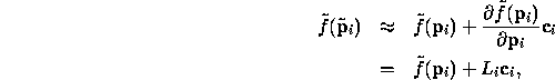
Since the 1-step errors are assumed to be small,
.
Since the 1-step errors are assumed to be small,
![]() is small. That is,
is small. That is, ![]() is close to a zero of g, if one
exists. A zero of the function would represent an orbit with zero
1-step error, i.e., a true orbit.
This is an ideal situation in which to run Newton's method.
If Newton's method converges, then a true orbit has been found.
is close to a zero of g, if one
exists. A zero of the function would represent an orbit with zero
1-step error, i.e., a true orbit.
This is an ideal situation in which to run Newton's method.
If Newton's method converges, then a true orbit has been found.
There are exactly two criteria for a trajectory ![]() to be
called a numerical shadow of
to be
called a numerical shadow of ![]() :
:
This section presents the GHYS refinement procedure for a two-dimensional
Hamiltonian system.
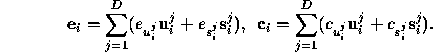
Assume we have a noisy orbit ![]() , and we want
to find a less noisy orbit
, and we want
to find a less noisy orbit ![]() . The 1-step
errors are estimated by
. The 1-step
errors are estimated by
![]()
where ![]() is an integrator with higher accuracy than the one
used to compute
is an integrator with higher accuracy than the one
used to compute ![]() . The refined orbit will be constructed by
setting
. The refined orbit will be constructed by
setting
![]()
where ![]() is a correction term for step i. Now,
is a correction term for step i. Now,
![]()
Assuming the correction terms ![]() to be small, then
to be small, then
![]() can be expanded in a Taylor series
about
can be expanded in a Taylor series
about ![]() :
:
where ![]() is
the linearized map. For a discrete chaotic map,
is
the linearized map. For a discrete chaotic map, ![]() is just the Jacobian of the map at step i.
For a system of ODEs,
is just the Jacobian of the map at step i.
For a system of ODEs,
![]() is the Jacobian of the integral of the ODE from step i to
step i+1.
is the Jacobian of the integral of the ODE from step i to
step i+1.![]() The final equation for the corrections is
The final equation for the corrections is
As will be seen later, it is the computation of the linear maps ![]() ,
called resolvents, that
takes most of the CPU time during a refinement, because
the resolvent has
,
called resolvents, that
takes most of the CPU time during a refinement, because
the resolvent has ![]() terms in it, and it needs to be computed
to high accuracy. Presumably, if one is interested in
studying simpler high-dimensional systems, a chaotic map would be a
better choice than an ODE system, because no ODE integration is
needed.
terms in it, and it needs to be computed
to high accuracy. Presumably, if one is interested in
studying simpler high-dimensional systems, a chaotic map would be a
better choice than an ODE system, because no ODE integration is
needed.
If the problem were not chaotic, the correction
terms ![]() could be computed directly from equation 1.1. But
since
could be computed directly from equation 1.1. But
since ![]() will amplify any errors in
will amplify any errors in ![]() that occur near the
unstable direction, computing the
that occur near the
unstable direction, computing the ![]() 's by iterating
equation 1.1 quickly produces nothing but noise.
Therefore, GHYS suggest splitting
the error and correction terms into components in the stable (
's by iterating
equation 1.1 quickly produces nothing but noise.
Therefore, GHYS suggest splitting
the error and correction terms into components in the stable ( ![]() )
and unstable (
)
and unstable ( ![]() ) directions at each timestep:
) directions at each timestep:
Computing the unstable unit direction vectors is currently
done by initializing the unstable vector at time 0, ![]() , to an
arbitrary unit vector and iterating the linearized map forward with
, to an
arbitrary unit vector and iterating the linearized map forward with
Since ![]() magnifies any component that lies in the unstable direction,
and assuming we are not so unlucky to choose a
magnifies any component that lies in the unstable direction,
and assuming we are not so unlucky to choose a ![]() that lies
precisely along the stable direction, then
after a few e-folding times
that lies
precisely along the stable direction, then
after a few e-folding times ![]() will point roughly in
the actual unstable direction. Similarly, the stable unit direction vectors
will point roughly in
the actual unstable direction. Similarly, the stable unit direction vectors
![]() are computed by initializing
are computed by initializing ![]() to an arbitrary unit vector
and iterating backwards,
to an arbitrary unit vector
and iterating backwards,
where ![]() can be computed either by inverting
can be computed either by inverting ![]() , or by
integrating the variational equations backwards from step i+1 to
step i. The latter is far more expensive, but may be more reliable
in rare instances.
In any case, it is intended that
, or by
integrating the variational equations backwards from step i+1 to
step i. The latter is far more expensive, but may be more reliable
in rare instances.
In any case, it is intended that
![]() , the identity matrix. There may
be more efficient ways to compute the stable and unstable vectors,
possibly having to do with eigenvector decomposition of the Jacobian
of the map (not the Jacobian of the integral of the map), but
I have not looked into this.
, the identity matrix. There may
be more efficient ways to compute the stable and unstable vectors,
possibly having to do with eigenvector decomposition of the Jacobian
of the map (not the Jacobian of the integral of the map), but
I have not looked into this.
Substituting equations 1.2 and 1.3 into equation 1.1 yields
For the same reason that ![]() magnifies errors in the unstable direction,
it diminishes errors in the stable direction. Likewise,
magnifies errors in the unstable direction,
it diminishes errors in the stable direction. Likewise, ![]() diminishes errors in the unstable direction and magnifies errors in the
stable direction. Thus the
diminishes errors in the unstable direction and magnifies errors in the
stable direction. Thus the ![]() terms should be computed
in the backwards direction, and
terms should be computed
in the backwards direction, and ![]() terms in the forward
direction. Taking components of equation 1.6
in the unstable direction at step i+1 (recall that
terms in the forward
direction. Taking components of equation 1.6
in the unstable direction at step i+1 (recall that ![]() lies in the same direction as
lies in the same direction as ![]() ), iterate backwards on
), iterate backwards on
and taking components in the stable direction, iterate forwards on
The initial choices for ![]() and
and ![]() are arbitrary as long
as they are small -- smaller than the maximum shadowing distance --
because equation 1.8 damps initial conditions, and
equation 1.7 damps final conditions. QT and
GHYS choose them both as 0. This choice is probably as good as any,
but it can be seen here that if one shadow exists, there are infinitely
many of them. (Another justification of this is offered below.)
Another way of looking at these initial choices
for
are arbitrary as long
as they are small -- smaller than the maximum shadowing distance --
because equation 1.8 damps initial conditions, and
equation 1.7 damps final conditions. QT and
GHYS choose them both as 0. This choice is probably as good as any,
but it can be seen here that if one shadow exists, there are infinitely
many of them. (Another justification of this is offered below.)
Another way of looking at these initial choices
for ![]() and
and ![]() is that they ``pinch'' the growing
components at the final end point, and the backwards-growing components
at the initial point, to be small, so that
is that they ``pinch'' the growing
components at the final end point, and the backwards-growing components
at the initial point, to be small, so that
![]() and
and ![]() .
That is, boundary conditions are being forced
on the problem so that the exponential
divergence is forcibly masked, if possible.
.
That is, boundary conditions are being forced
on the problem so that the exponential
divergence is forcibly masked, if possible.
Note that these boundary conditions allow the initial conditions for the shadow and noisy orbits to differ along the unstable direction. In fact, this must occur if the change in initial conditions is to have any effect. That is, when looking for a shadow, if perturbations are only allowed in the stable direction, those perturbations would die out, leading the ``shadow'' to follow the true orbit that passes through our initial conditions -- the one that is already known to diverge exponentially from the computed (noisy) orbit.
This section is derived from QT's Appendix B, although it is presented slightly differently.
If the configuration space is D dimensional, then there are 2D
dimensions in the phase space. It can be shown that in a Hamiltonian
system, the number of stable and unstable directions is each equal to D.
At timestep i, let ![]() be the D unstable unit vectors,
and let
be the D unstable unit vectors,
and let ![]() be the D stable unit vectors.
For any particular timestep,
it will be convenient if the unstable vectors are orthogonal to each other,
and the stable vectors are orthogonal to each other. However, the stable
and unstable vectors together will not in general form an orthogonal system.
be the D stable unit vectors.
For any particular timestep,
it will be convenient if the unstable vectors are orthogonal to each other,
and the stable vectors are orthogonal to each other. However, the stable
and unstable vectors together will not in general form an orthogonal system.
The vectors are evolved exactly as before, except using Gram-Schmidt
orthonormalization to produce two sets of D-orthonormal vectors at each
timestep.
Since we do not know a priori what directions are stable and
unstable at each timestep,
we choose an arbitrary orthonormal basis ![]() at time zero,
and an arbitrary orthonormal basis
at time zero,
and an arbitrary orthonormal basis ![]() at time S, and evolve them as:
at time S, and evolve them as:
![]()
Then, at each timestep i, do two Gram-Schmidt
orthonormalizations: one on ![]() to produce
to produce ![]() ,
and another on
,
and another on ![]() to produce
to produce ![]() . After a few e-folding times, we find that
. After a few e-folding times, we find that
![]() points in the most unstable direction at timestep i,
points in the most unstable direction at timestep i,
![]() points in the second most unstable direction, etc.
Likewise,
points in the second most unstable direction, etc.
Likewise, ![]() points in the most stable direction at time i,
points in the most stable direction at time i,
![]() points in the second most stable direction, etc.
points in the second most stable direction, etc.
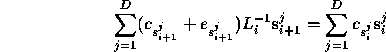
The multidimensional generalizations of the error and correction vectors is the obvious
To convert the 1-step error at timestep i from phase-space co-ordinates
![]() to the stable and unstable basis
to the stable and unstable basis
![]() ,
one constructs the matrix
,
one constructs the matrix ![]() whose columns are the unstable and stable
unit vectors,
whose columns are the unstable and stable
unit vectors, ![]() ,
and solves the system
,
and solves the system ![]() .
.
The equation for the correction co-efficients in the unstable subspace at timestep i+1 is
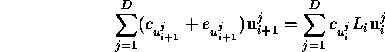
which we project out along ![]() producing
producing
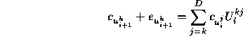
where the scalar ![]() , and the Gram-Schmidt process
ensures
, and the Gram-Schmidt process
ensures ![]() if j<k.
The boundary condition at timestep S is
if j<k.
The boundary condition at timestep S is ![]() ,
and we compute the co-efficients backwards using
,
and we compute the co-efficients backwards using
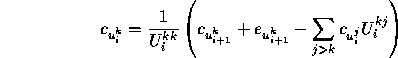
We first solve for ![]() , which doesn't require knowledge
of the other
, which doesn't require knowledge
of the other ![]() co-efficients, then we solve for
co-efficients, then we solve for ![]() ,
etc.
,
etc.
The equation for the correction co-efficients in the stable subspace at timestep i is
which we project out along ![]() producing
producing
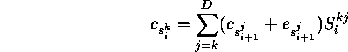
where ![]() , and the Gram-Schmidt process ensures
, and the Gram-Schmidt process ensures ![]() if j<k.
The boundary condition at time 0 is
if j<k.
The boundary condition at time 0 is ![]() ,
and we compute the co-efficients forwards using
,
and we compute the co-efficients forwards using
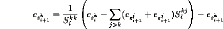
As with the unstable corrections, we first compute ![]() which does not require knowledge of the other
which does not require knowledge of the other ![]() co-efficients, then
we compute
co-efficients, then
we compute ![]() , etc.
, etc.
There is no guarantee that refinement converges towards a
true orbit; if there was, then all noisy orbits would be shadowable.
In fact, even if some refinements are successful,
numerical refinement alone does not prove rigorously that
a true shadow exists; it only proves the existence of
a numerical shadow, i.e., a trajectory that
has less noise than the original. Furthermore,
the 1-step error ![]() computed by any numerical technique
measures the difference between the noisy and
more accurate solutions at timestep i+1, where both start from the same
position at timestep i.
Even if this distance is about
computed by any numerical technique
measures the difference between the noisy and
more accurate solutions at timestep i+1, where both start from the same
position at timestep i.
Even if this distance is about ![]() ,
it does not imply that the difference between the noisy solution at
timestep i+1
and the true solution passing through step i is equally small.
This was
dramatically demonstrated one day when I accidentally set the precision
of the ``accurate'' integrator to only
,
it does not imply that the difference between the noisy solution at
timestep i+1
and the true solution passing through step i is equally small.
This was
dramatically demonstrated one day when I accidentally set the precision
of the ``accurate'' integrator to only ![]() , and the shadowing
routine happily refined the orbit until the 1-step errors
all had magnitudes less than
, and the shadowing
routine happily refined the orbit until the 1-step errors
all had magnitudes less than ![]() . Considering that the ``accurate''
trajectories were only being computed to a tolerance of
. Considering that the ``accurate''
trajectories were only being computed to a tolerance of ![]() , it seems
that refinement had converged to within
, it seems
that refinement had converged to within ![]() of a specific
numerical orbit that had true 1-step errors of about
of a specific
numerical orbit that had true 1-step errors of about ![]() .
.
Furthermore, a numerical integration routine that is requested to integrate
to a tolerance close to the machine precision might not achieve it,
because it might undetectably lose a few digits near the machine precision.
Thus, even when a numerical shadow is found with 1-step errors of
![]() , the true 1-step errors are probably closer to
, the true 1-step errors are probably closer to ![]() .
GHYS provide
a method called containment that can prove rigorously when
a true shadow exists, but we have not implemented containment.
As a surrogate to containment,
QT did experiments on simple chaotic maps with 100-digit accuracy
(using the Maple symbolic manipulation package) showing that if the
GHYS refinement procedure refined the trajectory to 1-step errors of about
.
GHYS provide
a method called containment that can prove rigorously when
a true shadow exists, but we have not implemented containment.
As a surrogate to containment,
QT did experiments on simple chaotic maps with 100-digit accuracy
(using the Maple symbolic manipulation package) showing that if the
GHYS refinement procedure refined the trajectory to 1-step errors of about
![]() , then successful refinements
could be continued down to
, then successful refinements
could be continued down to ![]() . It is reasonable to
assume that refinement would continue to decrease the
noise, converging in the limit to a noiseless (true) trajectory.
. It is reasonable to
assume that refinement would continue to decrease the
noise, converging in the limit to a noiseless (true) trajectory.
For the above reasons, we are confident that convergence to a numerical shadow implies, with high probability, the existence of a true shadow. However, to prove it rigorously requires implementing a scheme such as the GHYS containment procedure. This is one possible avenue for further research.
There is also no guarantee that, even if the refinement procedure
does converge, that it converges to a reasonable shadow of
![]() ; in principle it could converge to a true orbit that is far
from
; in principle it could converge to a true orbit that is far
from ![]() ,
in which case the term ``shadow'' would be inappropriate.
However, I have found in practice that refinement always fails
due to the 1-step errors ``exploding'' (becoming large).
I have never seen a case in which the refined orbit diverged from
the original orbit while retaining small 1-step errors.
,
in which case the term ``shadow'' would be inappropriate.
However, I have found in practice that refinement always fails
due to the 1-step errors ``exploding'' (becoming large).
I have never seen a case in which the refined orbit diverged from
the original orbit while retaining small 1-step errors.
The error explosion occurs when 1-step errors are so large that the linearized map becomes invalid for computing corrections. Since the method is global (i.e., each correction depends on all the others), inaccuracies in the computation of the corrections can quickly amplify the noise rather than decreasing it. Thus, within 1 or 2 refinement iterations, the 1-step errors can grow by many orders of magnitude, resulting in failed refinements. It is unclear if local methods like SLES (introduced below) will suffer the same consequences; probably they do, but errors probably grow much more slowly, and only locally in the orbit where 1-step errors are large.
I have tried two integrators as my ``accurate''
integrator, although both were variable-order,
variable-timestep Adams's methods
called SDRIV2 and LSODE [18, 16].
QT used a Bulirsch-Stoer integrator by Press et al. [28].
It would be interesting to study
whether the choice of accurate integrator influences the numerical
shadow found, because if one true shadow exists,
then infinitely many (closely packed) true shadows exist.![]() However, if the boundary conditions
are the same, then the solutions should be the same.
However, if the boundary conditions
are the same, then the solutions should be the same.
Since ![]() is arbitrary, and the displacement along
the actual unstable subspace at time 0 that determines the evolution
of the orbit, is it possible that we may fail to find a shadow because
the initial perturbations allowed by our choice of
is arbitrary, and the displacement along
the actual unstable subspace at time 0 that determines the evolution
of the orbit, is it possible that we may fail to find a shadow because
the initial perturbations allowed by our choice of ![]() don't
include the perturbations necessary to find a shadow?
don't
include the perturbations necessary to find a shadow?
I have not pursued this question at all, but it seems an interesting
one. There are examples introduced below where the GHYS refinement
procedure failed to find a shadow for a noisy orbit ![]() ,
when it can be shown that one exists;
the above scenario may be a cause. One way to test it is to try
to find a shadow for
,
when it can be shown that one exists;
the above scenario may be a cause. One way to test it is to try
to find a shadow for ![]() using a different initial guess for
using a different initial guess for ![]() ,
although I have not tried this. Similar comments apply to
,
although I have not tried this. Similar comments apply to ![]() .
.
However, there are at least 3 arguments against this dependence being
a problem. First, since the stable subspace has measure zero in the
total space, it seems unlikely that an arbitrary choice for
![]() could choose a subspace that doesn't contain ``enough'' of
the unstable subspace. Secondly, the correction co-efficients for
the unstable subspace are computed starting at the end of the
trajectory, where
could choose a subspace that doesn't contain ``enough'' of
the unstable subspace. Secondly, the correction co-efficients for
the unstable subspace are computed starting at the end of the
trajectory, where ![]() is presumably correct; similarly for the
correction co-efficients in the stable subspace and
is presumably correct; similarly for the
correction co-efficients in the stable subspace and ![]() . Thirdly,
assuming the shadowing distance is much larger than the 1-step errors,
it is likely that the intervals near the endpoints where the
stable/unstable vectors are inaccurate are too small to allow
instabilities in the computations of the corrections to build from 1-step
error sizes to shadow-distance sizes. Further
study of this possible problem may be helpful.
. Thirdly,
assuming the shadowing distance is much larger than the 1-step errors,
it is likely that the intervals near the endpoints where the
stable/unstable vectors are inaccurate are too small to allow
instabilities in the computations of the corrections to build from 1-step
error sizes to shadow-distance sizes. Further
study of this possible problem may be helpful.
If it does turn out to be a problem, there are many possible fixes. First, we could attempt to shadow only between points that are known to have accurate approximations to the stable and unstable directions. One measure of this accuracy is to start with two different arbitrary unit vectors at time 0 and evolve them forward using equation 1.4. When they converge within some tolerance to the same vector at timestep a, we can assume they are correct after timestep a. The same could be done to the stable vectors, starting with two different guesses at time S and evolving backwards using equation 1.5 until they converged at timestep b. Then, shadowing would be attempted only between a and b.
If we want to shadow all the way to the endpoints,
we could attempt to get reliable stable/unstable vectors everywhere in the
following manner:
compute the times a and b as above.
Then compute ![]() backwards, attempting to
evolve the correct
backwards, attempting to
evolve the correct ![]() backwards, while hoping that
instabilities from the stable subspace don't overwhelm the computation
for the few steps that iteration proceeds backwards.
Do the same for
backwards, while hoping that
instabilities from the stable subspace don't overwhelm the computation
for the few steps that iteration proceeds backwards.
Do the same for ![]() , except evolving forward. This seems to me the most
promising method, although I have not yet tested it. To test how much
of the unstable subspace has encroached on
, except evolving forward. This seems to me the most
promising method, although I have not yet tested it. To test how much
of the unstable subspace has encroached on ![]() , perhaps we
can dot
, perhaps we
can dot ![]() with
with ![]() to ensure it stays small.
to ensure it stays small.
Another (untested) method to compute the stable and unstable vectors out
to the endpoints is:
compute ![]() in the normal way. Then
choose
in the normal way. Then
choose ![]() to be orthogonal to
to be orthogonal to ![]() . Even though these vectors
are not generally orthogonal, choosing
. Even though these vectors
are not generally orthogonal, choosing ![]() to be orthogonal to
to be orthogonal to ![]() seems better than a random choice. Then, compute
seems better than a random choice. Then, compute ![]() normally. Then recompute
normally. Then recompute ![]() using a
using a ![]() orthogonal
to
orthogonal
to ![]() .
.
If a method can be invented that computes the stable and unstable vectors using eigenvector decomposition, then it probably would be better than all the above methods, because it would not require any resolvents and not be restricted to being away from the endpoints.