As described in the previous chapter, Grebogi, Hammel, Yorke, and Sauer (GHYS) [11], invented a two-dimensional shadowing procedure consisting of two parts:
Quinlan and Tremaine (QT) [29], wanted to test for the
existence of shadows in large N-body systems.
They generalized the
refinement portion of the GHYS algorithm to work on arbitrary-dimensional
Hamiltonian systems.
QT showed that, using 100 decimal digits of precision,
if the noise level of a four-dimensional orbit
could be reduced to about ![]() ,
then the noise could also be reduced all the way down to
,
then the noise could also be reduced all the way down to ![]() ,
with the number of correct digits in the solution increasing
geometrically.
They conclude that it is reasonable to assume that further refinement would
continue to reduce the noise indefinitely, leading in the limit to a true
orbit. This seems less rigourous that containment, but in practice
it is probably almost as reliable.
,
with the number of correct digits in the solution increasing
geometrically.
They conclude that it is reasonable to assume that further refinement would
continue to reduce the noise indefinitely, leading in the limit to a true
orbit. This seems less rigourous that containment, but in practice
it is probably almost as reliable.
QT then applied their refinement procedure to a simplified N-body
system in which a single particle moves, unsoftened, among 100 fixed particles
that are distributed in a standard Plummer distribution.
For their ``cheap'' integrator, they used a 5th-order predictor-corrector
routine that is commonly used by astronomers
[Appendix B of [6]], arranged to have 1-step errors
of about ![]() .
For their expensive integrator, they used a Bulirsch-Stoer method [28]
with tolerance
.
For their expensive integrator, they used a Bulirsch-Stoer method [28]
with tolerance ![]() .
They found they could shadow the particle for several crossing times.
Unfortunately, their refinement procedure was too inefficient
to work on significantly higher dimensional systems. They tried two and three
moving particles, but found they were pushing the bounds of feasibility
that their shadowing procedure could handle.
.
They found they could shadow the particle for several crossing times.
Unfortunately, their refinement procedure was too inefficient
to work on significantly higher dimensional systems. They tried two and three
moving particles, but found they were pushing the bounds of feasibility
that their shadowing procedure could handle.
It is perhaps important to note before continuing that it is not clear that refinement alone, even if optimized as introduced in this chapter, and even if it is as reliable as containment, is more efficient than using containment. But if refinement is to be used at all, it needs to be made more efficient than the direct, naïve method of GHYS and QT.
It is not at all clear that being able to shadow one particle moving
``pinball'' fashion amongst 100 fixed ones implies that
shadows of large N-body systems exist.
To establish the shadowability of large N-body simulations
requires shadowing tests to be applied to more realistic systems.
At present it is far beyond feasibility to attempt shadowing
systems of ![]() or
or ![]() particles that are commonly being
used today by astronomers.
Nevertheless, we can learn much about how shadowing
results change as the dimension increases,
using systems with just tens of moving particles.
In such systems it may be reasonable
to eliminate the fixed particles entirely, but to
extend QT's results, most of the experiments performed in
this thesis (and reported in the next chapter) were done on a system
with a total of 100 particles, M of which move, for M ranging from
1 to 25.
particles that are commonly being
used today by astronomers.
Nevertheless, we can learn much about how shadowing
results change as the dimension increases,
using systems with just tens of moving particles.
In such systems it may be reasonable
to eliminate the fixed particles entirely, but to
extend QT's results, most of the experiments performed in
this thesis (and reported in the next chapter) were done on a system
with a total of 100 particles, M of which move, for M ranging from
1 to 25.
It is important to emphasize the main scientific question that we will be studying once we have a reasonably fast shadowing implementation. The question is not only a question concerning N-body systems, but a general question for chaotic systems: how do shadowing results change as the number of dimensions increases?
For the remainder of this thesis, the following definitions will be in effect:
As has already been mentioned, most of the
expense of refinement of an N-body orbit is in computing the
linear maps ![]() .
See a previous footnote
for an explanation of
.
See a previous footnote
for an explanation of ![]() , and the Appendix for the derivation of
the Jacobian of an N-body system.
Manually counting floating-point operations in the Jacobian gives an
operation count of roughly
, and the Appendix for the derivation of
the Jacobian of an N-body system.
Manually counting floating-point operations in the Jacobian gives an
operation count of roughly ![]() . The total operation count
to compute the right hand side of the variational equation, including
the matrix-matrix multiply and the computation of the Jacobian, is
about
. The total operation count
to compute the right hand side of the variational equation, including
the matrix-matrix multiply and the computation of the Jacobian, is
about ![]() . The
. The ![]() term is probably negligible,
and the MN term is only relevant if N >> M.
Thus, if there are S shadow steps, and the function computing the
right hand side is invoked an
average of k times per shadow step,
the total cost of computing all the
resolvents is about
term is probably negligible,
and the MN term is only relevant if N >> M.
Thus, if there are S shadow steps, and the function computing the
right hand side is invoked an
average of k times per shadow step,
the total cost of computing all the
resolvents is about ![]() .
I have found
empirically that, using an Adams's integrator,
k seems to be independent of M, and roughly equal
to about 500 for the shadow steps I use in my N-body simulations.
Figure 2.0 shows some experiments comparing the time
to compute one resolvent to M, demonstrating the
.
I have found
empirically that, using an Adams's integrator,
k seems to be independent of M, and roughly equal
to about 500 for the shadow steps I use in my N-body simulations.
Figure 2.0 shows some experiments comparing the time
to compute one resolvent to M, demonstrating the ![]() relationship.
relationship.
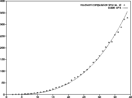
Figure 2.0: Time in seconds to compute one resolvent as a function of the
number of moving particles M. For comparison, ![]() is also plotted.
is also plotted.